Elizabeth Huang

Professor Carolyn Anderson

CS 232 Artificial Intelligence

9 May 2024

Geographic Trends in Industry Segmentation

1. Introduction

        When choosing an office location for a company, an assumption many company owners make is that they should locate their company within the radius (in close proximity) to its respective industry peers. However, in many circumstances, the most optimal location to be placed in depends on a multitude of other factors including supply, demand, regulations, etc.

        Previous research in this area solidifies the idea of a correlation between industry and geographic placement and defines a need for further research in the clustering of certain industries to particular geographic regions. A paper from the Institute for Research on Labor and Employment (Leung) performs an examination on occupational agglomeration (clustering) to observe the relationship between skill sets and geographic location. The paper mentions that current research suggests that industries tend to cluster geographically, which creates a need for a particular employee profile in particular geographic regions. Thus, particular industries and types of work become associated with geographic locations, creating a categorical stereotype or “spatial signaling.” Leung’s theory is that given a desired job category and country, a candidate from a desired country/ location will receive the job over any other candidate. Leung develops the following hypothesis: 1) the stronger a job-specific geographic identity, the greater the appeal for a candidate from that geographic region will be, 2) this bias will be strengthened for individuals for no previous relevant job experiences, and 3) this bias will be weakened for recruiters with poor past experiences of a specific job and geographic intersection. To test these hypotheses, Leung uses logistic regression to predict the likelihood of a particular candidate being chosen (given a job listing). The results of the paper indicate a significant concentration of candidates from India, however, a candidate from India having a negative effect on being selected by a recruiter/ employer. Additionally, all hypotheses were supported.^[1] Furthermore, research suggests that on average, industry locations are more strongly clustered in the United States than in the European Union,^[2] which makes the United States a more attractive candidate for observation to observe this relationship. According to LinkedIn’s 2016 Global Trend report, geographic matching for each candidate is a priority for 40% of big companies worldwide (and 45% of small businesses).^[3] To further understand the relationship between industries and geographic attractiveness, I hypothesize that LLaMA will perpetuate industry-geograpic stereotypes due to frequency of location mentioned in media and training data.

2. Probe Task

To better understand any underlying geographic stereotypes and assumptions with industry locations, the focus of this probe task is to analyze any assumptions in geographic location based on industry segments that may reinforce any geographic stereotypes.

1. Construct

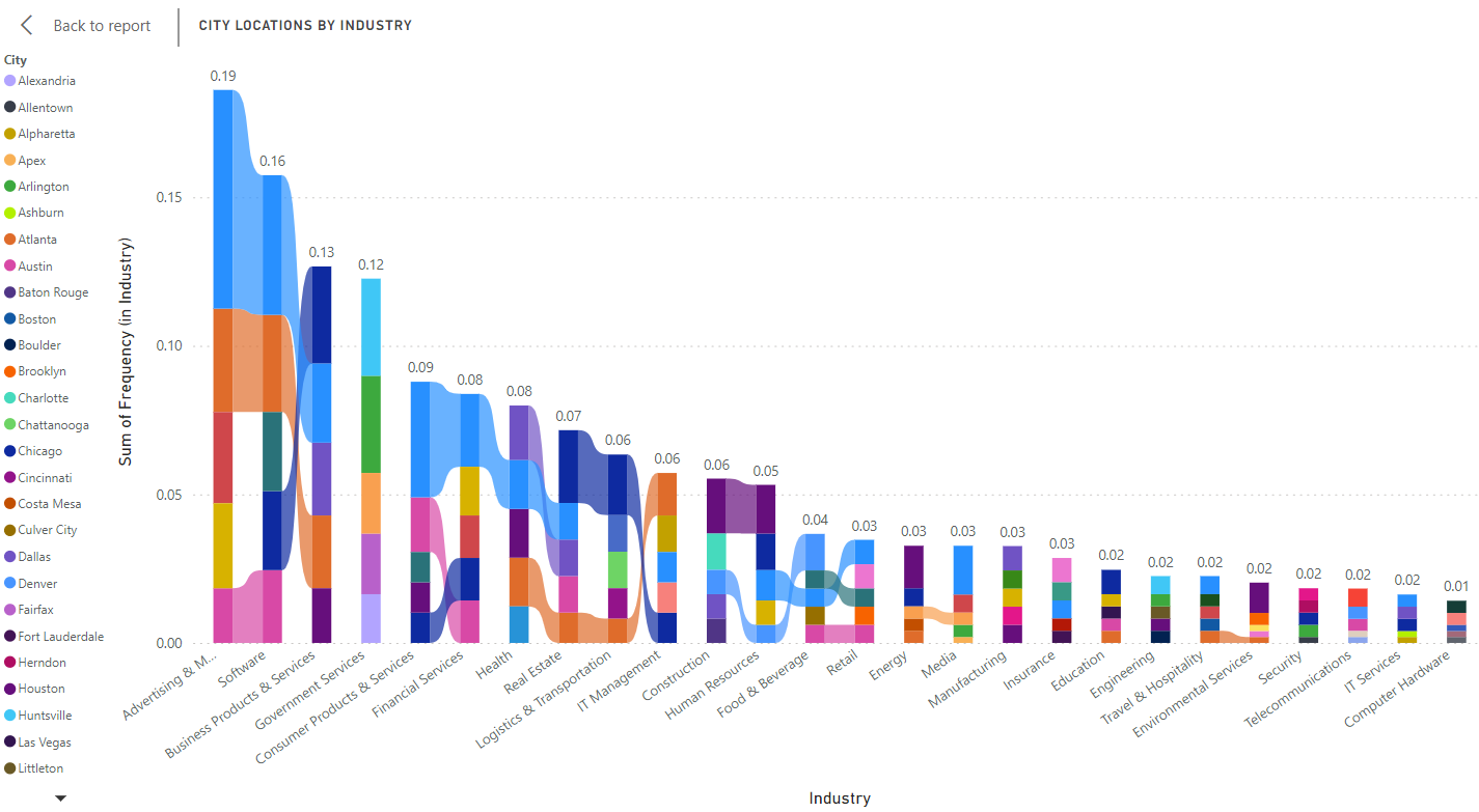
        The benchmark dataset used to test my hypothesis is the INC 500 (2019) list, which measures the frequency of geographic locations of the top 5,000 companies across various industries in the United States (Figure 1). This dataset is formatted to match the results of the model so we can compare the results of our model to the same standards as our baseline data. A summary of the most frequently appeared location for each industry in the initial dataset is reproduced below (Table 1).

Table 1: Cities with the highest frequency across each industry.

Figure 1: Visualization created from INC 5000 (2019) Dataset, Top 5 Cities in Each Industry Segment^[4]

2. Operationalization & Design Decisions

        To examine the hypothesis, the task can be operationalized with two sets of conditions and a set of frame sentences. The conditions used to probe the construct task include a set of 28 industry segments (Table 2, left side) extracted from the INC 5000 (2019) list with the addition of a neutral segment. Additionally, the top 24 states (Table 2, right side) form another set of conditions. With each industry segment and state, 18 frame sentences (Table 3) were used to form a total dataset of 9,222 usable outputs (cleaned and processed from 12,096 initial entries).

Table 2: Industry segment set (28) and US States set (24).

All 28 industry segments are taken from the observed set of industries in the raw dataset provided in the construct (see section 2.1). This is to ensure that the representation of the model’s output is representative of the actual range of industries and so that the metrics of the model’s dataset can be easily compared to that of the baseline. While there are 50 total states possible to choose from, due to running time constraints and the dataset size, I restricted the model’s range to the top 50% of most frequent states as ordered by the baseline dataset. Lastly, the frame sentences use different company type, stage, and working condition variants as the object is to observe the relationship between geographic locations and industry regardless of those factors. Besides minimal modifications to the descriptions of the company, all frame sentences alternate between the 28 industry segments and 24 possible states.

Table 4: Frame sentences (18).

3. Goal & Model Assessment

The overall goal of my probe task will be to evaluate accuracy metrics of the raw dataset (per industry segment) to the geographic viersity and centralization of the dataset of auto-completed cities. More specifically, I’ll be measuring the success of the model by comparing each overlap of cities in both the raw dataset and the LLaMA dataset, generated from using completion_query to evaluate centralization and accuracy will be evaluated on the top 5 most frequently appeared cities in each dataset with the following methods.

4. Metric Evaluation

         The success of the model will be determined by the following metrics: 1) the correlation of geography to industries in the resulting dataset, 2) number of overlapped cities per industry, and 3) the predicted distribution of cities and industries compared to the actual distribution. Bias is identified by checking for an inequitable distribution of data on one particular industry over another. There may also be geographic industry stereotypes (specific states or locations being known negatively for one particular industry over another based off of dense media coverage or over representation in the dataset).

3. Results

        On average, the model can predict 23.07% of the top 5 cities for any given industry, with the highest overlap of the top 5 cities in prediction being the Health industry with an accuracy of 60%. This analysis was done by comparing the top 5 cities per industry of the completion_query dataset to the top 5 cities per industry of the raw dataset. The correlation between industry and geographic location can be found by computing the Pearson coefficient, which is approximately 0.577641305. In other words, there is a medium, positive correlation between a city’s location and its industry. And we find that the similarity, which can be measured with a Jaccard coefficient, of the raw dataset to the generated dataset is roughly 0.394831383.

Table 5: Summary of best and worst performances and highest frequency neutral results.

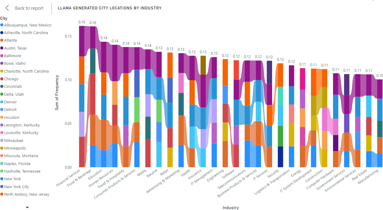
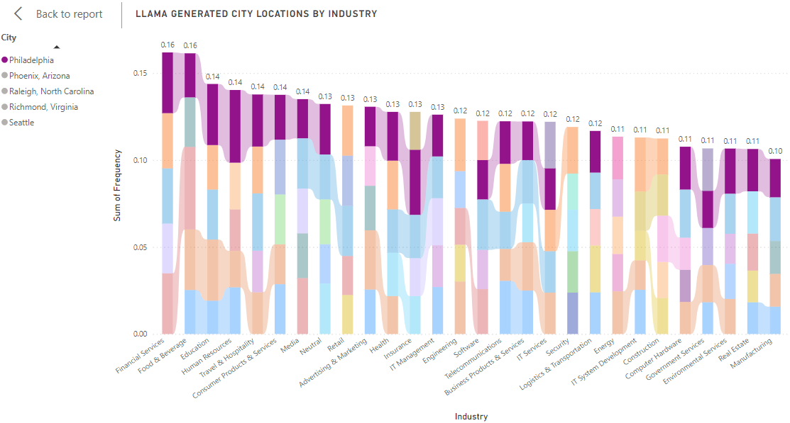
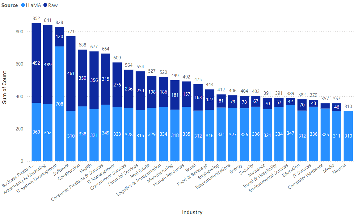
The overall representation of each industry segment and the most frequently resulting cities (Figure 2A) indicates a surprising trend. Among the top 5 cities generated for each industry, Philadelphia nearly appears in the top 5 list of every industry listed (Figure 2B). In the Neutral results, we can see Philidelphia listed within the top 5 cities as well (at a frequency of 2.90%), suggesting a possible bias or skew towards Philadelphia over any other city. On observation of the geographic distribution, there are two key details to note: 1) a spike in the number of IT System Development cities in the LLaMA dataset, and 2) an uneven distribution of cities in the raw dataset, with a large concentration of cities in the Business Product Managemnet industry and the smallest concentration of cities in the raw dataset for the Computer Hardware industry.

Overall, the probe task somewhat accurately measures the relationship between cities and industries. While the Pearson coefficient score is positive and above 0.5, a stronger positive correlation would likely produce more accurate results. A possible reasoning for the lower correlation coefficient score could be due to the lack of equitable distribution in the number of cities for each industry. Additionally, since the model used sentence completion rather than directly computing the likelihood or probabilities of particular cities, there is an accuracy loss in the resulting output. Sentence completion also required the use of heavy data cleaning to ensure that all data entries were geographic locations and not qualitative descriptions that could not be analyzed, losing about 3,000 entries in the dataset. Since the overlap of the generated dataset is roughly 40% similar to the raw dataset, it may imply an accuracy of human assumptions to the actual dataset, however, this accuracy is unclear without stronger correlation and more data. Furthermore, since the raw dataset is taken from 2019, current geographic trends may differ significantly from those used in the baseline comparison; a more recent dataset could likely demonstrate a stronger accuracy and performance.

Figure 2A: Visualization created from LLaMA Generation Prompts, Top 5 Cities in Each Industry Segment

Figure 2B: Visualization created from LLaMA Generation Prompts, Top 5 Cities in Each Industry Segment, Philadelphia Spotlighted

Figure 3: Visualization of City Distribution by Industry in LLaMA vs Raw Datasets

4. Conclusion

The probe task provided a somewhat accurate measure of the relationship between cities and industries. A key improvement that could be made on iteration of this project would be to use a more recent dataset as a baseline comparison and use word_query rather than completion_query to directly compare probabilities of the model to the raw dataset. Due to the selected operationalizaiton, the sentence completion of the designed prompts, incurred data cleaning losses (about 3,000 entries). From the selected dataset, there was also an uneven distribution of cities across industries, which may have measured the model’s performance inaccurately and inadvertently given rise to a representational harm in understanding the role of location for industries. In brief, this project analyzes the association between cities and industries, and can be further improved with more robust data and refined methodologies.

Bibliography

Abbot, L., Batty, R., Bevegni, S., Cuevas, A., Gager, S., Gordon, N., Hastings, K., & Stites, E. (n.d.). Global recruiting trends 2016. https://business.linkedin.com/content/dam/business/talent-solutions/global/en_us/c/pdfs/GRT16_GlobalRecruiting_100815.pdf

Ellison, Glenn, and Edward L., Glaeser. "The Geographic Concentration of Industry: Does Natural Advantage Explain Agglomeration?".American Economic Review 89, no.2 (1999): 311-316.

Inc. n.d. “Inc. 5000 List 2019.” https://www.inc.com/inc5000/2019. Cleaned in https://www.kaggle.com/datasets/mysarahmadbhat/inc-5000-companies/data

Leung, M. D. (2012). Job Categories and Geographic Identity: A Category Stereotype Explanation for Occupational Agglomeration. UC Berkeley: Institute for Research on Labor and Employment. Retrieved from https://escholarship.org/uc/item/31b4c6p8